The ARRAYFORMULA function runs a calculation over a whole range and writes the whole answer from one cell. Instead of a formula copied into two hundred rows, there is one formula, and it covers rows that do not exist yet.
That last part is the reason to care. A filled-down column is a snapshot of how tall the data was when somebody dragged it, so the first row appended past that point comes out blank and nothing complains.
This site appends rows from PHP, which is exactly the case that breaks a filled-down column. Append Google Sheets Rows Using Google Sheets API PHP Client adds rows to the bottom of a sheet on a schedule, and any calculated column beside them has to already cover the new rows or the script has to write those too. One open-ended array formula removes that whole problem.
There is one habit to learn with it, and skipping it is why people try the ARRAYFORMULA function once and go back to filling down. It is in step 3.
Requirements for the ARRAYFORMULA function:
- A Google Sheet you can edit
- A table with a header row
- Nothing to install, because the ARRAYFORMULA function ships with Google Sheets
Step 1.
First, the table this works on, in A1:D8.
Item      Qty   Price   Region
Widget    120   9.99    North
Gadget    45    24.50   South
Widget    120   9.99    North
Doohick   300   1.75    North
Gizmo     12    99.00   South
Gadget    80    24.50   East
Sprocket  5     3.25    North
The goal is a revenue column: quantity times price, for every row. Done the usual way that is one formula in the first row, then a drag to the bottom.
=B2 * C2
Step 2.
Next, do the whole column at once. Give the same expression ranges instead of single cells, and wrap it.
=ARRAYFORMULA(B2:B8 * C2:C8)
One cell holds the formula and seven cells fill with results. Delete the formula and all seven clear together, because there was only ever one calculation. Consequently there is no way for row 5 to quietly hold a different formula from row 4, which is the most common bug in a filled-down column.
Step 3.
Then extend it past the data, and meet the problem that has to be solved.
=ARRAYFORMULA(B2:B12 * C2:C12)
The range now runs to row 12, four rows below the last item. Those four rows are empty, and empty times empty is zero, so the column ends in zeros that look like real answers. Point it at B2:B instead, meaning the entire column, and you get a thousand of them.
=ARRAYFORMULA(IF(A2:A12 = "", "", B2:B12 * C2:C12))
The IF is the habit. Test a column that is only populated on real rows, return an empty string when it is blank, and calculate otherwise. Therefore the formula can cover far more rows than currently exist without printing anything for them, which is precisely what makes it survive an append.
Step 4.
Now use it for things that are not arithmetic. Anything that works on one row works on the range.
=ARRAYFORMULA(IF(A2:A8 = "", "", IF(B2:B8 > 100, "bulk", "small")))
=ARRAYFORMULA(IF(A2:A8 = "", "", TEXT(B2:B8 * C2:C8, "$#,##0.00")))
=ARRAYFORMULA(IF(A2:A8 = "", "", A2:A8 & " (" & D2:D8 & ")"))
Classification, formatting and concatenation all behave the same way. Note the second one in particular: TEXT returns a string, so this is how you get a formatted label rather than a formatted number, which matters when the result feeds a chart title or an email.
Step 5.
Finally, combine it with a lookup, which is where it saves the most work.
=ARRAYFORMULA(IF(A2:A8 = "", "", VLOOKUP(A2:A8, A2:C8, 3, FALSE)))
One lookup per row, all from one cell. Without the wrapper this returns a single value, because VLOOKUP expects one search key and quietly takes the first.
When Google asks for the ARRAYFORMULA function by name.
Some functions need the wrapper and say so. Try to total a calculated column without it:
=SUM(B2:B8 * C2:C8)
That returns #VALUE!, and the message behind it is unusually direct:
The default output of this reference is a single cell in the same
row but a matching value could not be found. To get the values for
the entire range use the ARRAYFORMULA function.
Wrapping it works, and so does the older idiom that has the array behaviour built in.
=ARRAYFORMULA(SUM(B2:B8 * C2:C8))
=SUMPRODUCT(B2:B8, C2:C8)
Both return the same total. SUMPRODUCT is shorter for this one case, while the wrapper generalises to anything, so learning the wrapper is the better investment.
Why the ARRAYFORMULA function beats filling down.
Three reasons, in the order they tend to matter.
It cannot drift. A filled-down column is many independent formulas, and any one of them can be overwritten by a paste without leaving a mark. One formula cannot disagree with itself.
It covers rows that do not exist yet. This is the one that pairs with a script: when an append adds rows, a filled-down column stops at whatever row somebody last dragged to, whereas an open-ended array formula has already covered them.
Finally, it makes the intent visible. Reading one formula tells you what the whole column means. Reading row 400 of a filled-down column tells you what row 400 means and leaves you to assume the rest.
Complete code for the ARRAYFORMULA function.
Every formula from this article, in order.
// One row at a time, the usual way.
=B2 * C2

// The whole range from one cell.
=ARRAYFORMULA(B2:B8 * C2:C8)

// Past the data, unguarded: the empty rows come out as zeros.
=ARRAYFORMULA(B2:B12 * C2:C12)

// Guarded, so empty rows stay empty. This is the form to use.
=ARRAYFORMULA(IF(A2:A12 = "", "", B2:B12 * C2:C12))

// It is not just arithmetic.
=ARRAYFORMULA(IF(A2:A8 = "", "", IF(B2:B8 > 100, "bulk", "small")))
=ARRAYFORMULA(IF(A2:A8 = "", "", TEXT(B2:B8 * C2:C8, "$#,##0.00")))
=ARRAYFORMULA(IF(A2:A8 = "", "", A2:A8 & " (" & D2:D8 & ")"))

// A lookup for every row, from one cell.
=ARRAYFORMULA(IF(A2:A8 = "", "", VLOOKUP(A2:A8, A2:C8, 3, FALSE)))

// SUM over a calculated range needs the wrapper, or SUMPRODUCT.
=SUM(B2:B8 * C2:C8)
=ARRAYFORMULA(SUM(B2:B8 * C2:C8))
=SUMPRODUCT(B2:B8, C2:C8)
Test the ARRAYFORMULA function.
Click an empty cell with room below it, paste a formula, and press Enter.
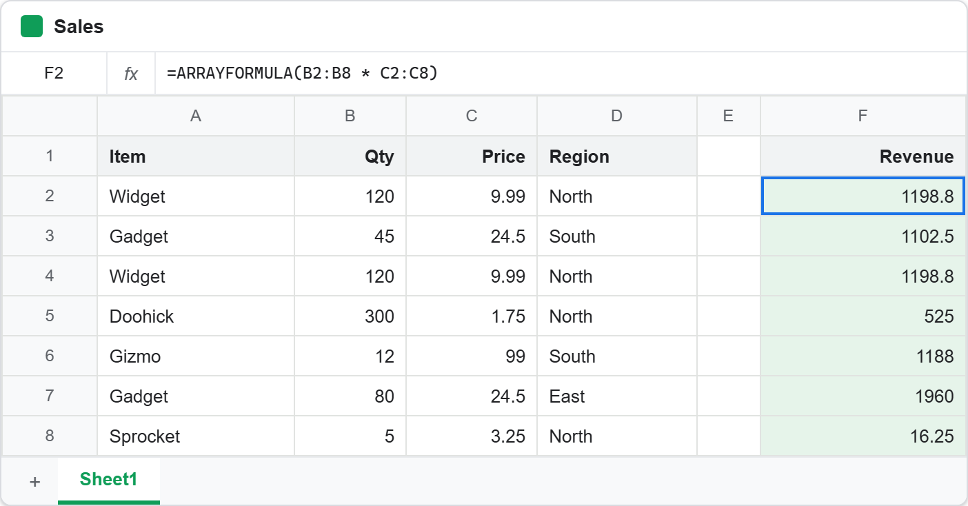
Click F1 -> paste the formula -> press Enter
Result of the ARRAYFORMULA function.
The wrapped version fills seven rows from one cell.
1198.8
1102.5
1198.8
525
1188
1960
16.25
Then the unguarded version shows the problem plainly. The same seven answers arrive, followed by three zeros for rows that hold nothing at all.
1198.8
1102.5
1198.8
525
1188
1960
16.25
0
0
0
Adding the IF guard removes them, and the output is identical to the tight range even though the formula covers five extra rows. Meanwhile the non-arithmetic examples show how far the idea stretches.
bulk           $1,198.80      Widget (North)
small          $1,102.50      Gadget (South)
bulk           $1,198.80      Widget (North)
bulk           $525.00        Doohick (North)
small          $1,188.00      Gizmo (South)
small          $1,960.00      Gadget (East)
small          $16.25         Sprocket (North)
Finally the total, which is the same either way.
=SUM(B2:B8 * C2:C8)                ->  #VALUE!
=ARRAYFORMULA(SUM(B2:B8 * C2:C8))  ->  7189.35
=SUMPRODUCT(B2:B8, C2:C8)          ->  7189.35
When to use the ARRAYFORMULA function.
Use it for any calculated column in a table that grows. That is most tables, and it is the whole argument in one sentence.
Skip it for a one-off calculation in a single cell, where the wrapper is noise. Skip it too when the column genuinely differs row by row, since an array formula exists to say that every row is treated the same way.
Above all, pair it with the guard. An open range without the IF is worse than filling down, because a column of zeros looks like data while an empty cell at least looks empty.