A grade scale, a shipping band or a commission tier is one question with several possible answers. The IFS function tests a list of conditions in order and returns the value paired with the first one that is true.
In fact, it replaces the nested IF, where each new band meant another IF inside the last one and another closing bracket at the end. With IFS, every test sits beside its answer in a single flat list.
However, IFS drops something the nested IF always had. There is no final “otherwise”, and a value that matches no test does not come back blank.
The IFS function.
So give it pairs: a test, then the value to return when that test is true.
=IFS(B2>=90,"A",B2>=80,"B",B2>=70,"C")
A score of 95 returns A, 82 returns B and 74 returns C. Excel reads the pairs from left to right and stops at the first true test, so it never looks at the rest.
Also, the order of the pairs is part of the logic. Written low to high, as =IFS(B2>=70,"C",B2>=80,"B",B2>=90,"A"), the first test catches everyone over 70, so the 95 gets a C as well. Therefore bands always go from the highest to the lowest.
There is no else.
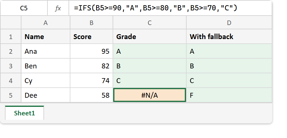
Next, look at the lowest score. Dee has 58, and none of the three tests is true for it.
As a result, the cell shows #N/A. Microsoft’s own reference says it plainly: when it finds no true condition, the IFS function returns #N/A. Nothing in the formula broke. It simply ran out of tests.
The fix is a last pair whose test is always true. Put TRUE where a condition would go, and that pair becomes the “otherwise”.
=IFS(B2>=90,"A",B2>=80,"B",B2>=70,"C",TRUE,"F")
Now 58 returns F. For example, use TRUE,"" instead when a non-match should simply stay empty.
Result of the IFS function.
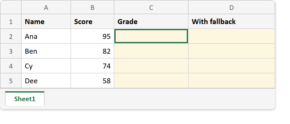
Before. Four names and four scores, with both grade columns empty.
After. The plain IFS function leaves Dee at #N/A, while the version with a TRUE fallback grades every row.
B2 -> 95    B3 -> 82    B4 -> 74    B5 -> 58

=IFS(B5>=90,"A",B5>=80,"B",B5>=70,"C")            ->  #N/A
=IFS(B5>=90,"A",B5>=80,"B",B5>=70,"C",TRUE,"F")   ->  F
=IFS(B2>=70,"C",B2>=80,"B",B2>=90,"A",TRUE,"F")   ->  C   (bands in the wrong order)
=IF(B5>=90,"A",IF(B5>=80,"B",IF(B5>=70,"C","F"))) ->  F   (the nested IF it replaces)
The IFS function needs Excel 2019 or later. For a single test with two outcomes, the plain IF function is still the shorter choice. And if you would rather catch the #N/A afterwards, IFERROR can do that, although the TRUE pair is clearer about what you meant.