One bad row turns a clean column into a wall of hash symbols. The IFERROR function swaps those for whatever you choose, and that convenience is also the trap.
Two functions do the work. IFERROR catches every error type there is, while IFNA catches only #N/A. In short, the distance between those two is the whole article.
Any formula that divides, looks up or parses will fail on some row eventually. A dashboard full of #DIV/0! is unreadable, so the instinct to hide them is right. However, the question is which ones you are hiding.
The IFERROR function.
Wrap the formula, then say what should appear when it fails.
=IFERROR(A2/B2,"")
Two arguments. The IFERROR function evaluates the first one, and if any error comes back it shows the second one instead.
An empty string is the usual second argument, because it leaves the cell looking blank. A short label such as "n/a" reads well too, and a zero works. Still, a zero then joins every average you take afterwards.
It catches your typos as well.
Here is the cost. It has no idea which errors you expected, so it swallows the ones that mean you made a mistake.
=IFNA(VLOOKUP(A2,Prices,2,FALSE),"")
Misspell a range name and the formula returns #NAME?. Wrap that in IFERROR and it becomes a blank cell, so the sheet looks finished while it is quietly wrong.
IFNA is the narrow version shown above. It catches #N/A and nothing else, which on a lookup is usually the only failure you actually planned for. Therefore your own mistakes still surface, still in red, still where you can see them.
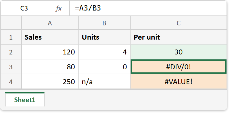
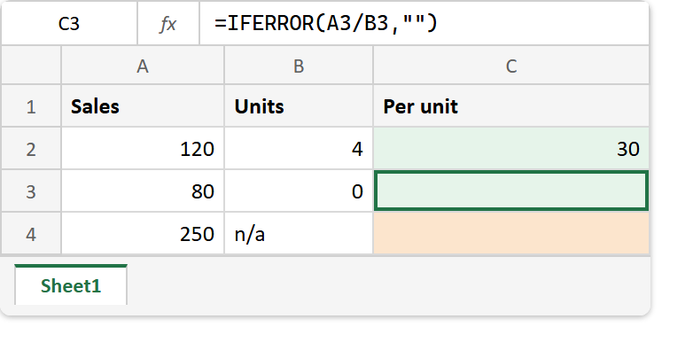
Result of the IFERROR function.
Before. The plain division, so two rows fail for two quite different reasons.
After. Both errors gone, both cells empty, and only the tint left to say that one of them was worth reading.
A2 / B2  ->  120 / 4      ->  30
A3 / B3  ->  80  / 0      ->  #DIV/0!
A4 / B4  ->  250 / "n/a"  ->  #VALUE!

=IFERROR(A3/B3,"")  ->  (blank)
=IFERROR(A4/B4,"")  ->  (blank)
Note the last two lines. Of course they look identical on the sheet, yet one was a divide by zero you knew about and the other is text sitting in a numeric column.
The blank those formulas leave behind is not an empty cell either, which is the next surprise waiting. COUNTA is what tells you so.