The SORTBY function returns a range in a new order, decided by a different range. You hand it the values you want to see and, separately, the values to sort them by. The second range never has to appear in the result. In fact, it does not even have to exist as a column, because a calculation works just as well.
The function takes the range to return, then one or more pairs of a sort key and a direction: 1 for ascending, -1 for descending. Its older sibling SORT can only sort by a column that is part of its own output, which is exactly the limit SORTBY removes. Along the way, TEXTBEFORE builds a key out of text. Then MATCH imposes an order that is not alphabetical at all.
This site also sorts from the other side. Create Xlsx Files With Auto Filter Settings gives a reader a filter arrow to click, so the sorting happens by hand inside the file. The SORTBY function instead returns the sorted rows as values, which is what you want when the result feeds another formula. Once you see that a sort key can be anything with the right number of rows, you will reach for it constantly.
Requirements for the SORTBY function:
- Excel 2021, Excel 2024, Microsoft 365, or Excel for the web
- A workbook you can edit
- Nothing to install, because the SORTBY function ships with Excel
SORTBY came with the dynamic array engine, so Excel 2021 runs it. However TEXTBEFORE, which appears in steps 4 and 5, arrived later — it needs Microsoft 365 or Excel 2024, and Excel 2021 answers #NAME? for it.
Step 1.
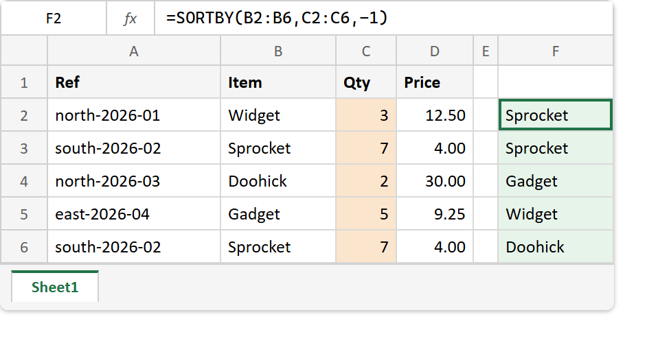
First, lay the table out in A1:D6. It is the same table as the rest of this group, so the results can be compared across articles.
Ref             Item      Qty   Price
north-2026-01   Widget    3     12.50
south-2026-02   Sprocket  7     4.00
north-2026-03   Doohick   2     30.00
east-2026-04    Gadget    5     9.25
south-2026-02   Sprocket  7     4.00
Step 2.
Next, sort the item names by quantity, largest first, without showing the quantity.
=SORTBY(B2:B6,C2:C6,-1)
Five names come back: Sprocket, Sprocket, Gadget, Widget, Doohick. The quantities decided that order, yet they are not in the result. Compare the same job done with SORT.
=SORT(B2:C6,2,-1)
That returns the identical order, but as two columns, because SORT can only sort by a column it is returning. To get the names alone you would have to wrap it in CHOOSECOLS. SORTBY simply never asks for the key column in the first place.
Step 3.
Then sort by something that is not a column at all. Revenue is quantity times price, and no cell holds it.
=SORTBY(B2:B6,C2:C6*D2:D6,-1)
The key is calculated inside the formula — 37.5, 28, 60, 46.25 and 28 — so the names come back as Doohick, Gadget, Widget, Sprocket, Sprocket. As a result there is no helper column to add, hide and forget about later.
Step 4.
Now sort by two keys. Each extra key is another pair of a range and a direction, read left to right.
=SORTBY(B2:C6,TEXTBEFORE(A2:A6,"-"),1,C2:C6,-1)
The first key is the region, cut from the front of each reference with TEXTBEFORE, so it too exists only inside the formula. The second key breaks ties within a region by quantity, highest first. The result is Gadget (east), then Widget and Doohick (north), then the two Sprocket rows (south).
Notice the two Sprocket rows tie on both keys. SORTBY is a stable sort, so rows that tie keep the order they had in the source. That matters more than it sounds, because it means a sort never shuffles equal rows at random between recalculations.
Step 5.
Finally, impose an order that is neither alphabetical nor numeric. Suppose the regions must read south, north, east.
=SORTBY(B2:B6,MATCH(TEXTBEFORE(A2:A6,"-"),{"south","north","east"},0),1)MATCH turns each region into its position in the list — 2, 1, 2, 3 and 1 — and SORTBY sorts by those numbers. Consequently the result is Sprocket, Sprocket, Widget, Doohick, Gadget. Change the list in the braces and the order changes with it, with no custom list to set up in Excel’s options.
The one mistake the SORTBY function will not forgive.
Every sort key must have exactly as many rows as the range being sorted. Make one a row short and the whole formula fails.
=SORTBY(B2:B6,C2:C5,-1)
That returns #VALUE!. It usually happens after a row is added to the table and only one of the two ranges is widened. Also note the direction is optional and defaults to ascending, so =SORTBY(B2:B6,C2:C6) quietly gives Doohick, Widget, Gadget, Sprocket, Sprocket — smallest quantity first. Type the -1 whenever you mean largest first.
When SORT is enough.
If the key is a column you want to show anyway, SORT is shorter and reads more plainly. The same holds when you already filter, dedupe and sort in one formula. This site covers that pattern for Google Sheets in Combine The FILTER Function With SORT And UNIQUE In Google Sheets. It works the same way in Excel.
=SORT(UNIQUE(FILTER(A2:D6,C2:C6>2)),3,-1)
That returns three whole rows — Sprocket, Gadget, Widget — with the duplicate Sprocket removed. Reach for SORTBY the moment the key is hidden, calculated, or more than one column.
Complete code for the SORTBY function.
Every formula from this article, in order.
// Step 2 - names by a quantity that is not shown, then SORT for contrast.
=SORTBY(B2:B6,C2:C6,-1)
=SORT(B2:C6,2,-1)

// Step 3 - a key calculated inside the formula.
=SORTBY(B2:B6,C2:C6*D2:D6,-1)

// Step 4 - two keys: region from the reference, then quantity.
=SORTBY(B2:C6,TEXTBEFORE(A2:A6,"-"),1,C2:C6,-1)

// Step 5 - a custom order, through MATCH.
=SORTBY(B2:B6,MATCH(TEXTBEFORE(A2:A6,"-"),{"south","north","east"},0),1)

// The mistake - keys of different sizes.
=SORTBY(B2:B6,C2:C5,-1)

// Whole rows, sorted by quantity.
=SORTBY(A2:D6,C2:C6,-1)

// When SORT is enough - filter, dedupe, sort by a visible column.
=SORT(UNIQUE(FILTER(A2:D6,C2:C6>2)),3,-1)
Test the SORTBY function.
Nothing to install. Click an empty cell, paste a formula, and press Enter.
Click F2 -> paste the formula -> press Enter
Result of the SORTBY function.
Sorting by a hidden column, then the same order from SORT with the key left in.
=SORTBY(B2:B6,C2:C6,-1)   ->  Sprocket
                              Sprocket
                              Gadget
                              Widget
                              Doohick

=SORT(B2:C6,2,-1)         ->  Sprocket  |  7
                              Sprocket  |  7
                              Gadget    |  5
                              Widget    |  3
                              Doohick   |  2
Next the calculated key, and the two-key sort.
=SORTBY(B2:B6,C2:C6*D2:D6,-1)                     ->  Doohick, Gadget, Widget, Sprocket, Sprocket

=SORTBY(B2:C6,TEXTBEFORE(A2:A6,"-"),1,C2:C6,-1)   ->  Gadget    |  5
                                                      Widget    |  3
                                                      Doohick   |  2
                                                      Sprocket  |  7
                                                      Sprocket  |  7
Then the custom order, the mistake, and the default direction.
=SORTBY(B2:B6,MATCH(TEXTBEFORE(A2:A6,"-"),{"south","north","east"},0),1)
                          ->  Sprocket, Sprocket, Widget, Doohick, Gadget

=SORTBY(B2:B6,C2:C5,-1)   ->  #VALUE!
=SORTBY(B2:B6,C2:C6)      ->  Doohick, Widget, Gadget, Sprocket, Sprocket
Finally, whole rows sorted by quantity.
=SORTBY(A2:D6,C2:C6,-1)   ->  south-2026-02  |  Sprocket  |  7  |  4
                              south-2026-02  |  Sprocket  |  7  |  4
                              east-2026-04   |  Gadget    |  5  |  9.25
                              north-2026-01  |  Widget    |  3  |  12.5
                              north-2026-03  |  Doohick   |  2  |  30
When to use the SORTBY function.
Use it whenever the order comes from something you do not want in the output. For example, that means a hidden column, a calculation, a code you cut apart first, or a priority list. Because the result is a live formula, it re-sorts itself the moment the data changes, and anything built on top of it follows.
Keep the sorting in code when a program is writing the workbook. Sort Rows Before Writing An Excel File In PHP Using PHPSpreadSheet orders the data before it ever reaches a cell. Meanwhile, the auto filter article hands the choice to the reader. Inside a workbook people keep editing, however, the SORTBY function is the better answer, because the order is a rule that survives them.