The FILTER function returns the rows that match a condition, and it returns them as a live block rather than a copy. Wrap it in UNIQUE and SORT and you have a small pipeline in one cell: keep these rows, drop the repeats, order what is left.
Each of the three is unremarkable alone. Composed, however, they stop looking like spreadsheet functions and start looking like a query, because the output of one becomes the input of the next. That is the same shape as chaining methods in code.
The PHP side of this site already does the other half of the job. Sort Rows Before Writing An Excel File In PHP Using PhpSpreadsheet orders the data in PHP and then writes it out. Here the sheet does the ordering itself, so the file on disk stays in whatever order it arrived.
Two things go wrong often enough to be worth naming up front. The FILTER function returns an error rather than a blank when nothing matches, and SORT counts its columns from the filtered result rather than from the sheet. Both are covered below.
Requirements for the FILTER function:
- A Google Sheet you can edit
- A table with a header row
- Nothing to install, because all three functions ship with Google Sheets
Step 1.
First, put the source table in A1:D8. Note the two identical Widget rows, since they are what UNIQUE has to work on later.
Item      Qty   Price   Region
Widget    120   9.99    North
Gadget    45    24.50   South
Widget    120   9.99    North
Doohick   300   1.75    North
Gizmo     12    99.00   South
Gadget    80    24.50   East
Sprocket  5     3.25    North
Step 2.
Next, keep only the rows you want. The FILTER function takes the range first, then a condition that has to be the same height as that range.
=FILTER(A2:D8, D2:D8 = "North")
That height rule is the one to internalise. A2:D8 is seven rows tall, so D2:D8 has to be seven rows tall as well. Consequently a condition written as D:D against a range of A2:D8 fails, because the two no longer line up.
Notice also that the header is excluded deliberately. The FILTER function has no header argument, unlike QUERY, so you point it at the data rows and nothing else.
Step 3.
Then narrow it further. Every extra argument is another condition, and they combine as AND.
=FILTER(A2:D8, D2:D8 = "North", B2:B8 > 50)
Sprocket drops out of the result here. It is in the North region, so it survived step 2, but its quantity of 5 fails the second test. Therefore adding conditions can only ever shrink the result, never grow it.
Step 4.
Now remove the duplicates. UNIQUE compares whole rows by default, not just the first column.
=UNIQUE(A2:D8)
This returns six rows out of seven. The two Widget rows are identical across all four columns, so one of them goes. Meanwhile the two Gadget rows both survive, because their quantities and regions differ.
That distinction matters more than it sounds. Point UNIQUE at a single column instead and you get the distinct values in it, which is the usual way to build a list of categories.
=UNIQUE(A2:A8)
Step 5.
Then order the result. SORT takes the range, a column number, and TRUE for ascending or FALSE for descending.
=SORT(A2:D8, 2, FALSE)
You can sort on more than one key by adding further triples. This one groups by region first, then puts the largest quantity at the top within each region.
=SORT(A2:D8, 4, TRUE, 2, FALSE)
Step 6.
Finally, compose all three. Read it inside out: filter first, then drop repeats, then sort what survives.
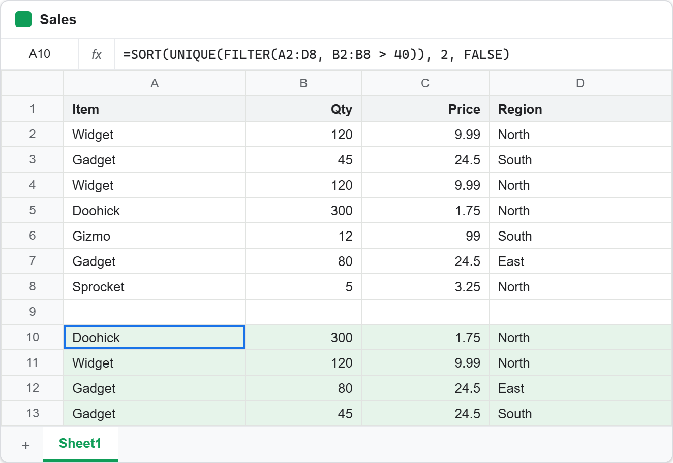
=SORT(UNIQUE(FILTER(A2:D8, B2:B8 > 40)), 2, FALSE)
Five rows pass the filter, one of them is a duplicate, and four come out sorted. Above all, note that nothing was written to the sheet in between. There is no helper column holding the filtered rows and no second column holding the deduplicated ones, so there is nothing to keep in step when the source data changes.
Sorting the output of the FILTER function.
Here is the trap. SORT’s column number counts across whatever it was handed, not across the sheet.
=SORT(FILTER(B2:D8, B2:B8 > 40), 1, FALSE)
The filter starts at column B this time, so the result has three columns, and column 1 of that result is the sheet’s column B. Ask for column 2 and you get Price rather than Quantity.
This is invisible when the filtered range happens to start at column A, which is why it usually bites later, after somebody edits the range. So count the columns in the FILTER function’s output, not on the sheet.
When the FILTER function finds nothing.
An empty result is not empty. It is an error.
=FILTER(A2:D8, D2:D8 = "West")
There is no West region in the table, so this returns #N/A. That is fine on its own, but it spreads: anything referring to this cell inherits the error, and a dashboard built on top of it fills with #N/A the moment a filter matches nothing.
=IFNA(FILTER(A2:D8, D2:D8 = "West"), "no rows")
Wrapping it in IFNA is the fix, and it costs nothing when the filter does match. Use it whenever the condition depends on data somebody else maintains, since the empty case will happen eventually.
Complete code for the FILTER function.
Every formula from this article. Each one needs empty cells to its right and below, because the results spill.
// Step 2 - keep the matching rows.
=FILTER(A2:D8, D2:D8 = "North")

// Step 3 - extra conditions are ANDed together.
=FILTER(A2:D8, D2:D8 = "North", B2:B8 > 50)

// Step 4 - distinct rows, then distinct values in one column.
=UNIQUE(A2:D8)
=UNIQUE(A2:A8)

// Step 5 - order by quantity, then by region and quantity.
=SORT(A2:D8, 2, FALSE)
=SORT(A2:D8, 4, TRUE, 2, FALSE)

// Step 6 - the three composed into one pipeline.
=SORT(UNIQUE(FILTER(A2:D8, B2:B8 > 40)), 2, FALSE)

// The index counts across the FILTER result, not the sheet.
=SORT(FILTER(B2:D8, B2:B8 > 40), 1, FALSE)

// An empty match is an error, so guard it.
=FILTER(A2:D8, D2:D8 = "West")
=IFNA(FILTER(A2:D8, D2:D8 = "West"), "no rows")
Test the FILTER function.
Nothing to install and nothing to run. Click an empty cell, paste a formula, and press Enter.
Click F1 -> paste the formula -> press Enter
Result of the FILTER function.
Step 2 keeps four of the seven rows, and both Widget rows come through because the filter has no opinion about duplicates.
Widget    120   9.99   North
Widget    120   9.99   North
Doohick   300   1.75   North
Sprocket  5     3.25   North
Then step 4 removes one of them. Six rows survive, and the pair of Gadget rows stays intact because they differ in quantity and region.
Widget    120   9.99    North
Gadget    45    24.5    South
Doohick   300   1.75    North
Gizmo     12    99      South
Gadget    80    24.5    East
Sprocket  5     3.25    North
The composed formula is the one worth reading twice. Five rows clear the quantity test, the duplicate Widget disappears, and the remainder come out largest first.
Doohick   300   1.75   North
Widget    120   9.99   North
Gadget    80    24.5   East
Gadget    45    24.5   South
Finally the two error cases, side by side. The bare filter reports a problem, while the guarded one reports an answer.
=FILTER(A2:D8, D2:D8 = "West")                    ->  #N/A
=IFNA(FILTER(A2:D8, D2:D8 = "West"), "no rows")   ->  no rows
When to use the FILTER function.
Reach for it when the rows you want are defined by a rule rather than by position. A rule keeps working after somebody inserts a row, whereas a hand-picked range does not.
Compose it with SORT and UNIQUE when the answer needs more than one step, and prefer that to helper columns. Helper columns work, but they have to be maintained, and they break quietly when the data grows past whatever range they were filled down to.
Reach for QUERY instead once you also want grouping or totals, since the FILTER function cannot aggregate. Reach for PHP when the result has to leave the sheet, which is what the Google Sheets API PHP client handles. The sheet is good at answering questions about itself, and a script is good at taking those answers somewhere else.