TAKE and DROP are opposites: TAKE returns the first or last few rows of a range, DROP returns everything except them. CHOOSECOLS and CHOOSEROWS pick specific ones by position. Together they let you carve a piece out of a range without writing a new range reference.
The reason that matters is that range references rot. Write A2:D6 today and it is wrong the moment somebody adds a row, whereas TAKE and DROP count from the edge of whatever the range currently holds.
This site slices from the other direction as well. Read Large Excel Files In Chunks In PHP Using PHPSpreadSheet takes a slice because the whole file will not fit in memory. Here we take a slice because the whole range is not the question — the same verb for an opposite reason.
One argument does most of the work in this article, and it is the one people never reach for: a negative count.
Requirements for TAKE and DROP:
- Microsoft 365, Excel 2024, or Excel for the web
- A workbook you can edit
- Nothing to install, because TAKE and DROP ship with Excel
Excel 2021 is not enough. It has dynamic arrays, so SORT and FILTER work there, but this family arrived later and Excel 2021 returns #NAME? for all four functions below.
Step 1.
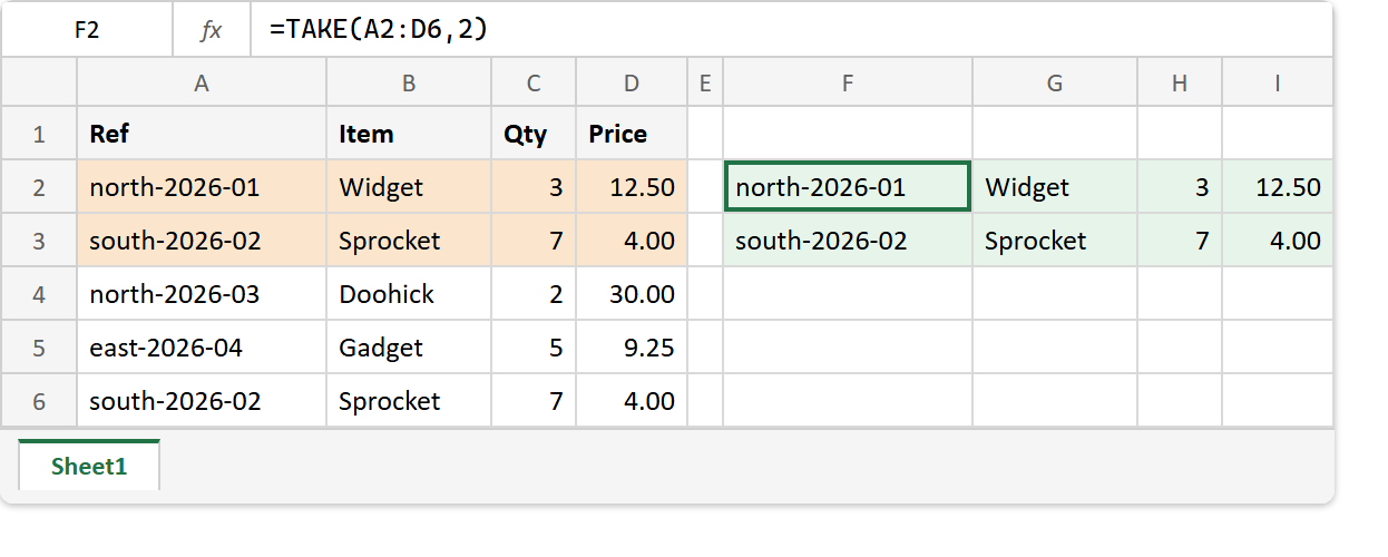
First, lay the table out in A1:D6. Five records, four columns, and a deliberate duplicate in the last row.
Ref             Item      Qty   Price
north-2026-01   Widget    3     12.50
south-2026-02   Sprocket  7     4.00
north-2026-03   Doohick   2     30.00
east-2026-04    Gadget    5     9.25
south-2026-02   Sprocket  7     4.00
Step 2.
Next, take the first rows. Two arguments: the range, and how many rows.
=TAKE(A2:D6,2)
Two complete records come back, all four columns intact. Notice that you did not have to work out that two rows means A2:D3 — the function counts for you, from the top of whatever it is given.
Step 3.
Then count from the other end. A negative number takes from the bottom instead.
=TAKE(A2:D6,-1)
That returns the last record. This is the single most useful thing here, because “the latest row” is a question every log, ledger and import sheet asks, and until now the answer involved INDEX and COUNTA and an off-by-one waiting to happen.
DROP works the same way in reverse.
=DROP(A2:D6,1)
=DROP(A2:D6,-2)
The first discards the top row and keeps four; the second discards the bottom two and keeps three. Consequently “everything except the header” and “everything except the totals” are both one short formula.
Step 4.
Now slice in both directions at once. The third argument does for columns what the second does for rows.
=TAKE(A2:D6,2,-2)
Two rows down, two columns in from the right — so the quantity and price of the first two records, without the reference or the item name. Because both counts are independent, any corner of a range is reachable with one call.
=DROP(A2:D6,0,-2)
Passing 0 for the rows keeps all of them while dropping the last two columns. Therefore 0 is how you say “leave this dimension alone”, rather than omitting the argument.
Step 5.
Finally, pick columns by position instead of by edge. CHOOSECOLS takes as many indexes as you like.
=CHOOSECOLS(A2:D6,2,4)
That returns the item name and the price, skipping the two columns between them. Also, the order you list the indexes is the order you get back, so this reorders as well as it selects.
=CHOOSECOLS(A2:D6,4,2)
Price first, then item. Negative indexes count from the right here too, and CHOOSEROWS is the same function applied to rows.
=CHOOSECOLS(A2:D6,-1)
=CHOOSEROWS(A2:D6,1,3)
What TAKE and DROP do that a fixed range cannot.
Compose it with a sort and the pattern that falls out is worth keeping.
=TAKE(SORT(A2:D6,3,-1),3)
Sort by the third column descending, then take the first three rows: a top-three list in one cell. Meanwhile the equivalent with fixed references needs a sorted helper block and a range that has to be widened by hand whenever the data grows.
One caveat on that particular result. The table contains a duplicate row, so the top three include Sprocket twice — which is correct, and a reminder that TAKE reports the data rather than tidying it. Wrap the sort in UNIQUE if distinct rows are what you meant.
An out-of-range index is an error rather than a silent empty.
=CHOOSECOLS(A2:D6,9)
That returns #VALUE!, since there is no ninth column. Note that asking TAKE for more rows than exist does not error — it simply returns everything, which is usually what you want and occasionally hides a mistake.
When INDEX still wins.
Two cases where the older function remains the right answer.
Use INDEX when you want one cell rather than a block, since these functions always return a range and a one-by-one range is an awkward thing to feed into text. Use it too when the workbook has to open in Excel 2021 or older, where INDEX has worked for thirty years and none of the four functions here exist.
Complete code for TAKE and DROP.
Every formula from this article, in order.
// Step 2 - the first rows.
=TAKE(A2:D6,2)

// Step 3 - a negative count works from the other end.
=TAKE(A2:D6,-1)
=DROP(A2:D6,1)
=DROP(A2:D6,-2)

// Step 4 - rows and columns in one call; 0 means "leave this alone".
=TAKE(A2:D6,2,-2)
=DROP(A2:D6,0,-2)

// Step 5 - pick columns by position, and reorder while picking.
=CHOOSECOLS(A2:D6,2,4)
=CHOOSECOLS(A2:D6,4,2)
=CHOOSECOLS(A2:D6,-1)
=CHOOSEROWS(A2:D6,1,3)

// Composed: the top three rows by quantity.
=TAKE(SORT(A2:D6,3,-1),3)

// An index that does not exist.
=CHOOSECOLS(A2:D6,9)
Test TAKE and DROP.
Nothing to install. Click an empty cell, paste a formula, and press Enter.
Click F2 -> paste the formula -> press Enter
Result of TAKE and DROP.
Taking from the top, and then from the bottom with a negative count.
=TAKE(A2:D6,2)    ->  north-2026-01  |  Widget    |  3  |  12.5
                      south-2026-02  |  Sprocket  |  7  |  4

=TAKE(A2:D6,-1)   ->  south-2026-02  |  Sprocket  |  7  |  4
Then the two DROP calls, which keep what TAKE would have discarded.
=DROP(A2:D6,1)    ->  4 rows, starting at south-2026-02
=DROP(A2:D6,-2)   ->  3 rows, ending at north-2026-03
Slicing both dimensions at once narrows the block to a corner.
=TAKE(A2:D6,2,-2)    ->  3  |  12.5
                         7  |  4

=DROP(A2:D6,0,-2)    ->  north-2026-01  |  Widget
                         south-2026-02  |  Sprocket
                         north-2026-03  |  Doohick
                         east-2026-04   |  Gadget
                         south-2026-02  |  Sprocket
Choosing columns by index, in the order given, then the same idea applied to rows.
=CHOOSECOLS(A2:D6,2,4)   ->  Widget | 12.5, Sprocket | 4, Doohick | 30, Gadget | 9.25, Sprocket | 4
=CHOOSECOLS(A2:D6,4,2)   ->  12.5 | Widget, 4 | Sprocket, 30 | Doohick, 9.25 | Gadget, 4 | Sprocket
=CHOOSECOLS(A2:D6,-1)    ->  12.5, 4, 30, 9.25, 4
=CHOOSEROWS(A2:D6,1,3)   ->  the north-2026-01 and north-2026-03 records
Finally the composed top-three, and the error an impossible index produces.
=TAKE(SORT(A2:D6,3,-1),3)   ->  south-2026-02  |  Sprocket  |  7  |  4
                                south-2026-02  |  Sprocket  |  7  |  4
                                east-2026-04   |  Gadget    |  5  |  9.25

=CHOOSECOLS(A2:D6,9)        ->  #VALUE!
When to use TAKE and DROP.
Use it any time the slice is defined relative to an edge — the latest entry, everything but the header, the last four quarters. Those definitions stay true as rows arrive, and a hard-coded range does not.
Keep the slicing in code when the constraint is memory rather than meaning, which is the case the PHPSpreadSheet article covers: a file too big to open is not a file you can put a formula in, and reading it in chunks is the only route. Once the data is small enough to sit in a workbook, TAKE and DROP express the slice more clearly than any range reference can.