Combine Ranges With The VSTACK And HSTACK Functions In Excel

VSTACK and HSTACK take several ranges and return them as one range: VSTACK stacks them one under the other, HSTACK lines them up sideways. Between them they replace the copy-paste-underneath routine that props up every monthly report.

The difference that matters is not the typing saved. A pasted block is a snapshot, so it is wrong the moment a source sheet changes, whereas VSTACK and HSTACK are live formulas that recombine every time anything underneath them moves.

This site solves the same problem from the other side as well. Copy A Worksheet Into Another Excel File In PHP Using PHPSpreadSheet physically copies a sheet from one workbook into another, which is right when a program is assembling the file. Here we combine ranges that are already in front of us and leave the originals alone.

One thing to watch throughout. Excel allows ranges of different shapes, and what it does about the gap is the single most useful thing in this article.

Requirements for VSTACK and HSTACK:

• Microsoft 365, Excel 2024, or Excel for the web
• A workbook you can edit
• Nothing to install, because VSTACK and HSTACK ship with Excel

Excel 2021 is not enough. It runs dynamic arrays, so SORT and UNIQUE work there, but the stacking family landed in a later wave and Excel 2021 answers #NAME?.

Step 1.

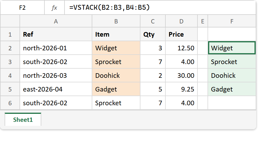
First, lay the table out in A1:D6. The last row repeats the second one exactly, which matters as soon as we start removing duplicates.

Ref             Item      Qty   Price
north-2026-01   Widget    3     12.50
south-2026-02   Sprocket  7     4.00
north-2026-03   Doohick   2     30.00
east-2026-04    Gadget    5     9.25
south-2026-02   Sprocket  7     4.00

Step 2.

Next, stack two ranges vertically. Each range is just another argument.

=VSTACK(B2:B3,B4:B5)

Four names come back in one column. In a real workbook those two arguments would be Jan!B2:B40 and Feb!B2:B36, and the point is the same: the ranges do not have to be adjacent, on the same sheet, or even the same length.

Step 3.

Then stack sideways instead. HSTACK lines ranges up shoulder to shoulder.

=HSTACK(B2:B4,C2:C4)

That rebuilds a two-column block from two separate one-column ranges. Consequently you can assemble a table from columns that live nowhere near each other, without moving any of them.

Step 4.

Now the combination that earns the whole article. Stack everything, then drop the repeats, in one formula.

=UNIQUE(VSTACK(B2:B6,B2:B6))

The inner call produces ten rows; the outer one returns four. Sorting is one more wrapper if you want the list stable rather than in first-seen order.

=SORT(UNIQUE(VSTACK(B2:B6,B2:B6)))

Therefore “combine twelve monthly sheets into one deduplicated, alphabetised list” is a single cell rather than a procedure. Because it is a formula, next month’s numbers flow through it the moment somebody types them.

Step 5.

Finally, stack whole rows rather than single columns. Any rectangular range works as an argument.

=VSTACK(A2:D3,A5:D5)

Three complete records come back, four columns wide, picked from two places in the table. That is the shape you want when the result feeds another formula rather than a human reader.

What VSTACK and HSTACK do with ranges that do not match.

This is the part worth knowing before you trust it with real data. Stacking ranges of different sizes does not fail — it pads.

=HSTACK(B2:B4,C2:C6)

The first range is three rows, the second is five, so the result runs to five rows and the two missing cells in the first column come back as #N/A. Notice that Excel highlights nothing and shows no warning. Meanwhile the errors are real errors, so anything referring to that block inherits them.

The fix is one wrapper, and it should be a habit rather than a repair.

=IFNA(HSTACK(B2:B4,C2:C6),"-")

Use IFNA rather than IFERROR here. The padding is specifically #N/A, and IFERROR would also swallow a genuine #DIV/0! arriving from the source data, which is exactly the error you want to keep seeing.

When copy and paste still wins.

There are three cases where the old routine is still the right answer.

Use paste when the combined block is a permanent record that must not change again — a closed quarter, an archived figure, anything that would go wrong if somebody edited a source later. Use it when you are about to delete the sources, since a formula pointing at a missing range returns #REF! while a pasted block simply survives. Finally, use it when the workbook has to open in Excel 2021 or older, where these functions do not exist.

Complete code for VSTACK and HSTACK.

Every formula from this article, in order.

// Step 2 - stack two ranges into one column.
=VSTACK(B2:B3,B4:B5)

// Step 3 - stack sideways instead.
=HSTACK(B2:B4,C2:C4)

// Step 4 - stack, then remove duplicates, then sort.
=UNIQUE(VSTACK(B2:B6,B2:B6))
=SORT(UNIQUE(VSTACK(B2:B6,B2:B6)))

// How many rows went in, before the dedupe.
=ROWS(VSTACK(B2:B6,B2:B6))

// Step 5 - stack whole four-column rows.
=VSTACK(A2:D3,A5:D5)

// Ranges of different lengths pad with #N/A.
=HSTACK(B2:B4,C2:C6)

// Catch the padding, but only the padding.
=IFNA(HSTACK(B2:B4,C2:C6),"-")

Test VSTACK and HSTACK.

Nothing to install. Click an empty cell, paste a formula, and press Enter.

Click F2  ->  paste the formula  ->  press Enter

Result of VSTACK and HSTACK.

The two simple stacks return the shapes you would draw by hand.

=VSTACK(B2:B3,B4:B5)     ->  Widget
                             Sprocket
                             Doohick
                             Gadget

=HSTACK(B2:B4,C2:C4)     ->  Widget    |  3
                             Sprocket  |  7
                             Doohick   |  2

Then the dedupe. Ten rows go in and four come out, and adding SORT changes only the order.

=ROWS(VSTACK(B2:B6,B2:B6))           ->  10
=UNIQUE(VSTACK(B2:B6,B2:B6))         ->  Widget, Sprocket, Doohick, Gadget
=SORT(UNIQUE(VSTACK(B2:B6,B2:B6)))   ->  Doohick, Gadget, Sprocket, Widget

Stacking whole rows keeps all four columns together.

north-2026-01  |  Widget    |  3  |  12.5
south-2026-02  |  Sprocket  |  7  |  4
east-2026-04   |  Gadget    |  5  |  9.25

Finally the mismatched stack, which is the one to look at closely. Excel pads the shorter range rather than rejecting it.

=HSTACK(B2:B4,C2:C6)             ->  Widget    |  3
                                     Sprocket  |  7
                                     Doohick   |  2
                                     #N/A      |  5
                                     #N/A      |  7

=IFNA(HSTACK(B2:B4,C2:C6),"-")   ->  the same block, with "-" in place of #N/A

When to use VSTACK and HSTACK.

Reach for it whenever the answer is “all of these ranges together” and people are still editing the ranges. It survives new rows, it survives new sheets if you point it at a whole column, and it composes with UNIQUE, SORT and FILTER without any glue.

Keep the assembly in code when a program is producing the workbook in the first place, which is what the PHPSpreadSheet article covers: a script that already has both sheets open can merge them before anyone opens the file, and the reader never sees the seam. Inside a workbook that people maintain by hand, the formula is better, because it shows where every row came from.

References: