This article shows how to set up conditional formatting in a Google Sheet from PHP: a rule that turns low stock numbers red, and a colour scale that shades a price column from light to dark. Both are one batchUpdate call.
The Excel half of this site covers the same ground twice, in cell conditional formatting settings and in data bars, colour scales and icon sets. Those posts split the subject into rules that test a value and rules that paint a spread across a range, and the Google Sheets API splits it the same way: booleanRule and gradientRule.
There is one thing to get straight before writing any of it. Conditional formatting in a Google Sheet is not a cell format. It is a rule stored on the sheet, and the cell is never touched — which changes how you check that your code worked.
Requirements for conditional formatting in a Google Sheet:
- Authenticate With A Service Account
- Create A Google Cloud Project
- Enable Google Sheets API Library
- Install The Google Client Library Specifying Google Sheets
- Composer
- PHP 8.1 or newer
Step 1.
First, set up the dependencies. This is the Sheets-only install used across this series. Tested with google/apiclient 2.19 on PHP 8.5.
{
    "require": {
        "google/apiclient": "^2.12.1"
    },
    "scripts": {
        "pre-autoload-dump": "Google\\Task\\Composer::cleanup"
    },
    "extra": {
        "google/apiclient-services": [
            "Sheets"
        ]
    }
}
Step 2.
Next, install the Google Client Library.
$ composer install
Step 3.
Then build the client and resolve the tab id, exactly as the other requests in this series do.
<?php

require 'vendor/autoload.php';

use Google\Client;
use Google\Service\Sheets;
use Google\Service\Sheets\BatchUpdateSpreadsheetRequest;
use Google\Service\Sheets\Request;
use Google\Service\Sheets\ValueRange;

$spreadsheetId = 'YOUR_SPREADSHEET_ID';
$keyFile = 'service-account.json';
$tabName = 'Stock';

$client = new Client();
$client->setApplicationName('Conditional Formatting');
$client->setAuthConfig($keyFile);
$client->addScope(Sheets::SPREADSHEETS);

$service = new Sheets($client);

$sheetId = sheetIdFor($service, $spreadsheetId, $tabName);
Step 4.
Clear any rules already on the tab. Rules accumulate: addConditionalFormatRule adds, it never replaces, so running a script twice leaves you with two copies of everything. Deleting index 0 until the API complains is the blunt, reliable way to start clean.
while (true) {
    try {
        $service->spreadsheets->batchUpdate($spreadsheetId, new BatchUpdateSpreadsheetRequest([
            'requests' => [
                new Request(['deleteConditionalFormatRule' => [
                    'sheetId' => $sheetId,
                    'index'   => 0,
                ]]),
            ],
        ]));
    } catch (Google\Service\Exception $e) {
        break;
    }
}
Rules are addressed by position, and deleting one renumbers everything after it. That is why this loop keeps asking for 0 rather than counting upwards.
Step 5.
Put some stock levels in, and define the two ranges the rules will watch.
$service->spreadsheets_values->update(
    $spreadsheetId,
    $tabName . '!A1',
    new ValueRange(['values' => [
        ['Item', 'In stock', 'Price'],
        ['Widget', 120, 9.99],
        ['Gadget', 45, 24.50],
        ['Doohick', 300, 1.75],
        ['Gizmo', 12, 99.00],
    ]]),
    ['valueInputOption' => 'USER_ENTERED']
);

$dataRange = [
    'sheetId'          => $sheetId,
    'startRowIndex'    => 1,
    'endRowIndex'      => 5,
    'startColumnIndex' => 1,
    'endColumnIndex'   => 2,
];

$priceRange = [
    'sheetId'          => $sheetId,
    'startRowIndex'    => 1,
    'endRowIndex'      => 5,
    'startColumnIndex' => 2,
    'endColumnIndex'   => 3,
];
Step 6.
The first rule tests a value. A booleanRule pairs one condition with one format, and the format is applied to any cell in the range where the condition holds.
$lowStock = new Request(['addConditionalFormatRule' => [
    'index' => 0,
    'rule'  => [
        'ranges'      => [$dataRange],
        'booleanRule' => [
            'condition' => [
                'type'   => 'NUMBER_LESS',
                'values' => [['userEnteredValue' => '50']],
            ],
            'format' => [
                'backgroundColor' => ['red' => 0.96, 'green' => 0.80, 'blue' => 0.80],
                'textFormat'      => ['bold' => true],
            ],
        ],
    ],
]]);
Note that the threshold is the string '50', not the integer 50. Condition values are always userEnteredValue strings, the same way a person would type them into the box, and that includes numbers and dates.
Step 7.
The second rule paints a spread instead of testing anything. A gradientRule has no condition at all — just an anchor at each end, and the API interpolates between them.
$priceScale = new Request(['addConditionalFormatRule' => [
    'index' => 1,
    'rule'  => [
        'ranges'       => [$priceRange],
        'gradientRule' => [
            'minpoint' => ['type' => 'MIN', 'color' => ['red' => 1.0, 'green' => 1.0, 'blue' => 1.0]],
            'maxpoint' => ['type' => 'MAX', 'color' => ['red' => 0.20, 'green' => 0.67, 'blue' => 0.28]],
        ],
    ],
]]);

$service->spreadsheets->batchUpdate($spreadsheetId, new BatchUpdateSpreadsheetRequest([
    'requests' => [$lowStock, $priceScale],
]));
MIN and MAX mean “whatever the smallest and largest values in the range turn out to be”, so the scale re-anchors itself when the data changes. Use NUMBER with a value instead when you want fixed ends, or PERCENTILE when outliers would otherwise flatten everything else.
Step 8.
Finally, read the rules back. They are not on the cells, so this reads the sheet.
$meta = $service->spreadsheets->get($spreadsheetId, [
    'fields' => 'sheets(properties(sheetId),conditionalFormats)',
]);

foreach ($meta->getSheets() as $sheet) {
    if ($sheet->getProperties()->getSheetId() !== $sheetId) {
        continue;
    }

    $rules = $sheet->getConditionalFormats() ?? [];
    printf("Rules stored on the tab: %d\n", count($rules));
}
Complete code for conditional formatting in a Google Sheet.
<?php

require 'vendor/autoload.php';

use Google\Client;
use Google\Service\Sheets;
use Google\Service\Sheets\BatchUpdateSpreadsheetRequest;
use Google\Service\Sheets\Request;
use Google\Service\Sheets\ValueRange;

$spreadsheetId = 'YOUR_SPREADSHEET_ID';
$keyFile = 'service-account.json';
$tabName = 'Stock';

$client = new Client();
$client->setApplicationName('Conditional Formatting');
$client->setAuthConfig($keyFile);
$client->addScope(Sheets::SPREADSHEETS);

$service = new Sheets($client);

function sheetIdFor(Sheets $service, string $spreadsheetId, string $title): int
{
    foreach ($service->spreadsheets->get($spreadsheetId)->getSheets() as $sheet) {
        if ($sheet->getProperties()->getTitle() === $title) {
            return $sheet->getProperties()->getSheetId();
        }
    }

    $service->spreadsheets->batchUpdate($spreadsheetId, new BatchUpdateSpreadsheetRequest([
        'requests' => [
            new Request(['addSheet' => ['properties' => ['title' => $title]]]),
        ],
    ]));

    return sheetIdFor($service, $spreadsheetId, $title);
}

$sheetId = sheetIdFor($service, $spreadsheetId, $tabName);

// Start from a clean tab so the rule list is not appended to on a re-run.
while (true) {
    try {
        $service->spreadsheets->batchUpdate($spreadsheetId, new BatchUpdateSpreadsheetRequest([
            'requests' => [
                new Request(['deleteConditionalFormatRule' => [
                    'sheetId' => $sheetId,
                    'index'   => 0,
                ]]),
            ],
        ]));
    } catch (Google\Service\Exception $e) {
        break;
    }
}

$service->spreadsheets_values->update(
    $spreadsheetId,
    $tabName . '!A1',
    new ValueRange(['values' => [
        ['Item', 'In stock', 'Price'],
        ['Widget', 120, 9.99],
        ['Gadget', 45, 24.50],
        ['Doohick', 300, 1.75],
        ['Gizmo', 12, 99.00],
    ]]),
    ['valueInputOption' => 'USER_ENTERED']
);

$dataRange = [
    'sheetId'          => $sheetId,
    'startRowIndex'    => 1,
    'endRowIndex'      => 5,
    'startColumnIndex' => 1,
    'endColumnIndex'   => 2,
];

$priceRange = [
    'sheetId'          => $sheetId,
    'startRowIndex'    => 1,
    'endRowIndex'      => 5,
    'startColumnIndex' => 2,
    'endColumnIndex'   => 3,
];

// A boolean rule: one condition, one format, applied when it is true.
$lowStock = new Request(['addConditionalFormatRule' => [
    'index' => 0,
    'rule'  => [
        'ranges'      => [$dataRange],
        'booleanRule' => [
            'condition' => [
                'type'   => 'NUMBER_LESS',
                'values' => [['userEnteredValue' => '50']],
            ],
            'format' => [
                'backgroundColor' => ['red' => 0.96, 'green' => 0.80, 'blue' => 0.80],
                'textFormat'      => ['bold' => true],
            ],
        ],
    ],
]]);

// A gradient rule: no condition, a colour scale across the range.
$priceScale = new Request(['addConditionalFormatRule' => [
    'index' => 1,
    'rule'  => [
        'ranges'       => [$priceRange],
        'gradientRule' => [
            'minpoint' => ['type' => 'MIN', 'color' => ['red' => 1.0, 'green' => 1.0, 'blue' => 1.0]],
            'maxpoint' => ['type' => 'MAX', 'color' => ['red' => 0.20, 'green' => 0.67, 'blue' => 0.28]],
        ],
    ],
]]);

$service->spreadsheets->batchUpdate($spreadsheetId, new BatchUpdateSpreadsheetRequest([
    'requests' => [$lowStock, $priceScale],
]));

echo "Rules applied.\n\n";

// Read the rules back. They live on the SHEET, not on the cells.
$meta = $service->spreadsheets->get($spreadsheetId, [
    'fields' => 'sheets(properties(sheetId),conditionalFormats)',
]);

foreach ($meta->getSheets() as $sheet) {
    if ($sheet->getProperties()->getSheetId() !== $sheetId) {
        continue;
    }

    $rules = $sheet->getConditionalFormats() ?? [];
    printf("Rules stored on the tab: %d\n", count($rules));

    foreach ($rules as $index => $rule) {
        if ($rule->getBooleanRule()) {
            $condition = $rule->getBooleanRule()->getCondition();
            $values = array_map(
                fn($value) => $value->getUserEnteredValue(),
                $condition->getValues() ?? []
            );
            printf("  [%d] boolean  %s %s\n", $index, $condition->getType(), implode(', ', $values));
        }

        if ($rule->getGradientRule()) {
            printf("  [%d] gradient %s -> %s\n", $index,
                $rule->getGradientRule()->getMinpoint()->getType(),
                $rule->getGradientRule()->getMaxpoint()->getType());
        }
    }
}

// Gizmo has 12 in stock, so the rule matches and B5 is pink on screen.
$cell = $service->spreadsheets->get($spreadsheetId, [
    'ranges'          => [$tabName . '!B5'],
    'includeGridData' => true,
    'fields'          => 'sheets(data(rowData(values(userEnteredFormat,effectiveFormat(backgroundColor)))))',
]);

$values = $cell->getSheets()[0]->getData()[0]->getRowData()[0]->getValues()[0];

echo "\nB5 holds 12, so the rule matches. What does the cell say?\n";
printf("  userEnteredFormat : %s\n", $values->getUserEnteredFormat() ? 'set' : 'none');

$effective = $values->getEffectiveFormat();
printf("  effectiveFormat   : %s\n", $effective ? sprintf('%.2f / %.2f / %.2f',
    $effective->getBackgroundColor()->getRed() ?? 0,
    $effective->getBackgroundColor()->getGreen() ?? 0,
    $effective->getBackgroundColor()->getBlue() ?? 0) : 'none');
Test the conditional formatting in a Google Sheet.
$ php conditional.php
Result of the conditional formatting in a Google Sheet.
Rules applied.

Rules stored on the tab: 2
  [0] boolean  NUMBER_LESS 50
  [1] gradient MIN -> MAX

B5 holds 12, so the rule matches. What does the cell say?
  userEnteredFormat : none
  effectiveFormat   : 0.96 / 0.80 / 0.80
The rule is not on the cell.
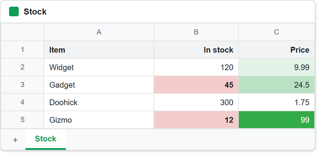
The last three lines are the ones to keep. B5 holds 12, the rule says anything under 50 goes pink, and on screen that cell is pink. Ask the cell about its formatting and you get two different answers depending on which question you ask.
userEnteredFormat is none, because nobody formatted that cell. Nothing was written to it, and the repeatCell request that formats cells directly was never involved. The rule lives on the sheet in conditionalFormats, as an ordered list, and it describes cells rather than belonging to them.
effectiveFormat is the pink. That is the cell’s appearance after every rule has been applied — what a person actually sees. So there are three things you can read, and they answer three different questions: the rule list says what rules exist, userEnteredFormat says what was written to the cell, and effectiveFormat says what the cell looks like now.
This matters because the obvious way to verify your work is the wrong one. Check userEnteredFormat after adding a rule and it reads none, which looks exactly like a request that silently failed. It did not fail; you asked the wrong question.
Add conditional formatting in a Google Sheet that survives a re-run.
Two habits keep this tidy. Always clear before you add, since rules accumulate and a script run three times paints three identical rules that all fire at once. And remember that rules are ordered: the first matching rule wins for a given property, so put your most specific rule at a lower index than the general one.
Beyond that the shape stays constant. A booleanRule when the answer is yes or no, a gradientRule when it is a spread, condition values as strings, and colours as floats from 0 to 1. If you need a rule that tests something the built-in condition types do not cover, CUSTOM_FORMULA takes an ordinary sheet formula written from the top-left cell of the range, and the rest of the request is unchanged.