The QUERY function lets you interrogate a Google Sheet the way you would interrogate a database. You write select, where, group by and order by inside a single cell, and the sheet answers with a block of results that updates itself whenever the source data changes.
That is a different way of working. Most spreadsheet answers are assembled from a stack of helper columns, with a FILTER here and a SUMIF there. However, the QUERY function collapses that stack into one readable string, so the logic sits in one place instead of being smeared across the grid.
This site already reads the same kind of data from the other side. Read Google Sheets Cells Using Google Sheets API PHP Client pulls a range into PHP and does the work there. Meanwhile the QUERY function does the equivalent job inside the sheet, which is often all you need. When it is not, the two combine, because a script can read the block a query produced just like any other range.
One trap catches nearly everybody once. Column references change shape depending on what you point the query at, and getting it wrong does not produce a helpful message. Instead you get a bare #N/A. Step 6 covers that in full, because it is the single most useful thing to know here.
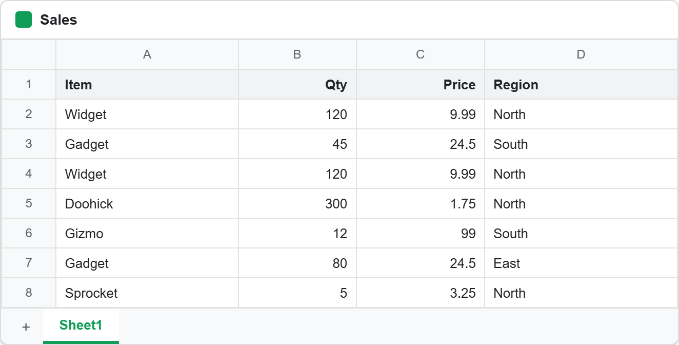
Seven rows, four columns, one deliberate duplicate. Notice that Widget appears twice with identical numbers, and that Region has three distinct values. Both details matter later.
Requirements for the QUERY function:
- A Google Sheet you can edit
- A table with a header row
- Nothing to install, because the QUERY function ships with Google Sheets
Step 1.
First, lay out the source table. Put it in A1:D8, with the header in row 1.
Item      Qty   Price   Region
Widget    120   9.99    North
Gadget    45    24.50   South
Widget    120   9.99    North
Doohick   300   1.75    North
Gizmo     12    99.00   South
Gadget    80    24.50   East
Sprocket  5     3.25    North
Any table works, so use your own if you prefer. The examples below all point at A1:D8, so adjust that reference to match whatever you actually have.
Step 2.
Next, pick some columns. This is the smallest useful query, and it introduces all three arguments at once.
=QUERY(A1:D8, "select A, B", 1)
The first argument is the range to read. The second is the query itself, written as a string. The third says how many rows of that range are headers, and it is the argument people leave out and then regret.
Pass 1 and the sheet knows row 1 is a header, so it labels the output and excludes it from the data. Leave it out entirely and Google guesses, which usually works and occasionally does not. Therefore it is worth stating explicitly every time.
Note that A and B here are the real column letters on the sheet. They are not positions inside the range, which is a distinction that becomes important in step 6.
Step 3.
Then filter the rows with where. It behaves the way it does in SQL, including the comparison operators.
=QUERY(A1:D8, "select A, B, D where D = 'North'", 1)
Look closely at the quoting, since this is where a first attempt usually breaks. The whole query is a string in double quotes, so any text you compare against has to use single quotes inside it. Consequently where D = "North" will not work, and the error it gives does not mention quoting at all.
Step 4.
Now sort and trim the result. Both clauses go inside the same string, and the order of the clauses matters.
=QUERY(A1:D8, "select A, B where B > 40 order by B desc limit 3", 1)
Clauses have to appear in SQL’s order: select, then where, then group by, then order by, then limit. Swap any two and the query fails. So if a query that looks right refuses to run, check the clause order before you check anything else.
Also notice that limit applies after the sort, not before it. As a result this returns the three largest quantities rather than the first three rows that happened to match.
Step 5.
Then aggregate. This is the point where the QUERY function stops being a fancy filter and starts doing work a helper column cannot do on its own.
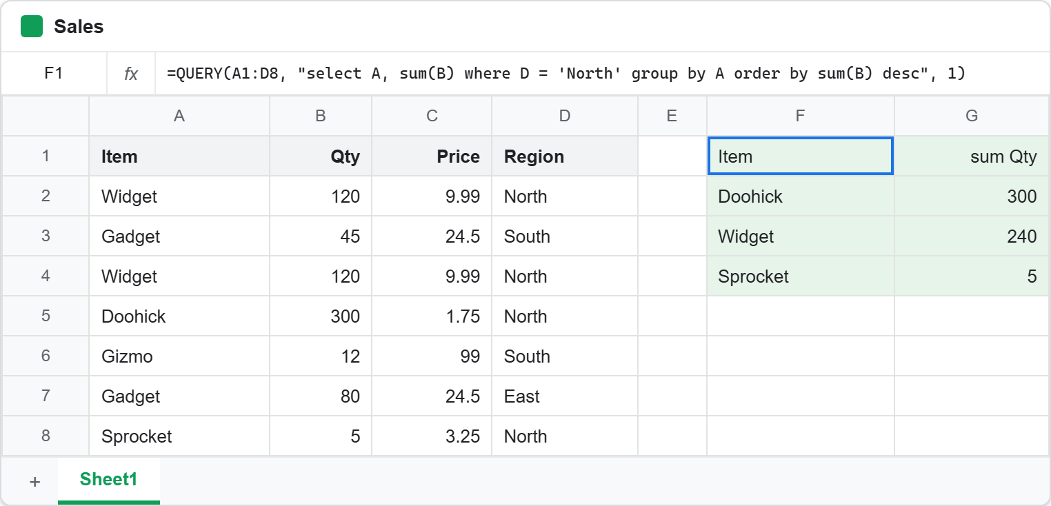
=QUERY(A1:D8, "select A, sum(B) where D = 'North' group by A order by sum(B) desc", 1)
That reads as one sentence: total the quantities per item, but only for the North region, and put the biggest first. Writing the same thing with SUMIF would need a list of unique items first, then a formula beside each one, then a sort. Here it is one cell.
The output has a detail worth pointing out. Google invents a header for the aggregated column and calls it sum Qty, which is not text you will find anywhere in the source data. If that generated name bothers you, rename it with a label clause.
=QUERY(A1:D8, "select A, sum(B) where D = 'North' group by A order by sum(B) desc label sum(B) 'Total units'", 1)
The label clause goes last and takes the aggregate exactly as you wrote it in the select. Above all, note that it repeats sum(B) rather than referring to the output column, which reads oddly the first time.
The column reference trap in the QUERY function.
Here is the thing that costs people an afternoon. How you name columns depends entirely on what you hand the query as its first argument.
Point it at a real range and you use the sheet’s column letters, as every example above does. Point it at an array instead, which is what curly braces build, and the letters stop meaning anything. Arrays have no column letters, so you refer to positions with Col1, Col2 and so on.
=QUERY({A2:D8}, "select Col1, Col2 where Col2 > 100", 0)That works. Now compare it with the identical query written the way habit suggests.
=QUERY({A2:D8}, "select A, B where B > 100", 0)That one returns #N/A and nothing else. Same data, same logic, same answer wanted, and the only difference is Col1 versus A.
Meanwhile the braces are genuinely the trigger, not the row range. Drop them and the letters work again straight away.
=QUERY(A2:D8, "select A, B where B > 100", 0)
So the rule is about the braces specifically. Anything built with {} is an array, and an array only understands Col1. That covers stacked ranges such as {A2:D8; A20:D30}, which is exactly when people reach for braces in the first place.
IMPORTRANGE deserves its own note, because it looks like it ought to behave as an array and does not. Both styles work there, yet they count differently. Import Sheet1!B1:D6 and the block keeps its original letters, so select B returns the first column you imported. Meanwhile Col1 counts from the start of the import, which makes Col1 and B the same column here. Ask for select A instead and the QUERY function answers NO_COLUMN: A, since column A was never part of the import.
Complete code for the QUERY function.
Every formula from this article, in order. Drop each one into an empty cell with room to its right and below, because the results spill.
// Step 2 - pick columns.
=QUERY(A1:D8, "select A, B", 1)

// Step 3 - filter rows. Single quotes inside the double-quoted query.
=QUERY(A1:D8, "select A, B, D where D = 'North'", 1)

// Step 4 - sort, then keep the top three.
=QUERY(A1:D8, "select A, B where B > 40 order by B desc limit 3", 1)

// Step 5 - total per item, biggest first.
=QUERY(A1:D8, "select A, sum(B) where D = 'North' group by A order by sum(B) desc", 1)

// Step 5 - the same thing with a readable header.
=QUERY(A1:D8, "select A, sum(B) where D = 'North' group by A order by sum(B) desc label sum(B) 'Total units'", 1)

// Step 6 - an array needs Col1, not A.
=QUERY({A2:D8}, "select Col1, Col2 where Col2 > 100", 0)

// Step 6 - the same query with letters against an array returns #N/A.
=QUERY({A2:D8}, "select A, B where B > 100", 0)

// Step 6 - without the braces, the letters work again.
=QUERY(A2:D8, "select A, B where B > 100", 0)
Test the QUERY function.
There is nothing to run and nothing to install. Click an empty cell, paste one formula, and press Enter.
Click F1 -> paste the formula -> press Enter
If a formula returns #REF! rather than data, the result had nowhere to spill into. Clear the cells below and to the right, then try again.
Result of the QUERY function.
Step 2 returns both columns with the header carried through, so the block is eight rows deep including that header.
Item      Qty
Widget    120
Gadget    45
Widget    120
Doohick   300
Gizmo     12
Gadget    80
Sprocket  5
Then step 4 sorts and trims, which is where the limit ordering shows up clearly. Doohick leads on 300, and the two Widget rows fill the rest because both hold 120.
Item      Qty
Doohick   300
Widget    120
Widget    120
Step 5 is the one worth studying. The two Widget rows have collapsed into a single total of 240, Gadget has gone entirely because neither of its rows is in the North region, and the header reads sum Qty.
Item      sum Qty
Doohick   300
Widget    240
Sprocket  5
Finally, the trap from step 6, side by side. The first query names its columns Col1 and Col2 and returns three rows. The second changes nothing except the column names and returns an error.
=QUERY({A2:D8}, "select Col1, Col2 where Col2 > 100", 0)
Widget    120
Widget    120
Doohick   300

=QUERY({A2:D8}, "select A, B where B > 100", 0)
#N/A
When to reach for the QUERY function.
Use it when the answer needs more than one operation. Filtering alone is FILTER’s job and sorting alone is SORT’s job, but as soon as you want to filter and group and sort together, stacking those functions gets hard to read while a query stays a sentence.
Use it too when somebody else has to maintain the sheet. A colleague can read select A, sum(B) where D = 'North' group by A and know what it does, even without knowing spreadsheets well. Three nested functions do not offer that.
Reach for something else when the job is genuinely one step, since =SUMIF(D2:D8, "North", B2:B8) is clearer than a query that only totals a column. Reach for PHP when the result has to leave the sheet, which is what the Google Sheets API PHP client is for. The two approaches answer the same question from opposite ends, and knowing both means you can pick per job rather than per habit.