The XLOOKUP function looks a value up in one range and returns the matching value from another. That sounds like VLOOKUP with a new name, but the two ranges are separate arguments rather than one block and a column number, and that single change removes most of the ways VLOOKUP goes wrong.
It also fails politely. VLOOKUP hands you #N/A and leaves you to wrap it in IFERROR, whereas the XLOOKUP function takes the fallback as an ordinary argument.
This site writes lookups from the other direction too. Use VLOOKUP In Excel Files In PHP Using PhpSpreadsheet generates a VLOOKUP into a file from PHP, which is still the right call when the file has to open in Excel. Here we are working inside the sheet instead, where the newer function is available.
One caveat before starting. This does not mean INDEX and MATCH are finished, and the section near the end says exactly when the older pair is still the better answer.
Requirements for the XLOOKUP function:
- A Google Sheet you can edit
- A table with a header row
- Nothing to install, because the XLOOKUP function ships with Google Sheets
Step 1.
First, lay out the table in A1:D8. Two rows share the item name Widget, which matters when we come to duplicate matches.
Item      Qty   Price   Region
Widget    120   9.99    North
Gadget    45    24.50   South
Widget    120   9.99    North
Doohick   300   1.75    North
Gizmo     12    99.00   South
Gadget    80    24.50   East
Sprocket  5     3.25    North
Step 2.
Next, the simplest lookup. Search for a value in one column, return from another.
=XLOOKUP("Gizmo", A2:A8, C2:C8)Three arguments: what to find, where to look, and what to return. There is no column number anywhere, so inserting a column between the two ranges cannot break this formula. That is the failure VLOOKUP is famous for, and it disappears here rather than being worked around.
Step 3.
Then handle the miss. Left alone, a failed search behaves like VLOOKUP’s.
=XLOOKUP("Nothing", A2:A8, C2:C8)That returns #N/A, which spreads into anything referring to it. However the fourth argument fixes it without any wrapping.
=XLOOKUP("Nothing", A2:A8, C2:C8, "not found")Consequently a sheet full of lookups stays readable. Compare that with =IFERROR(VLOOKUP(...), "not found"), where the interesting part sits in the middle and the fallback trails off the end.
Step 4.
Now return more than one value. Give the return argument several columns and the answer spills across.
=XLOOKUP("Gizmo", A2:A8, B2:D8)One formula produces the whole record rather than three formulas producing three cells. Therefore a row of details stays in step automatically, because there is only one lookup to be wrong.
Step 5.
Then search backwards through the columns, which is the thing VLOOKUP genuinely cannot do.
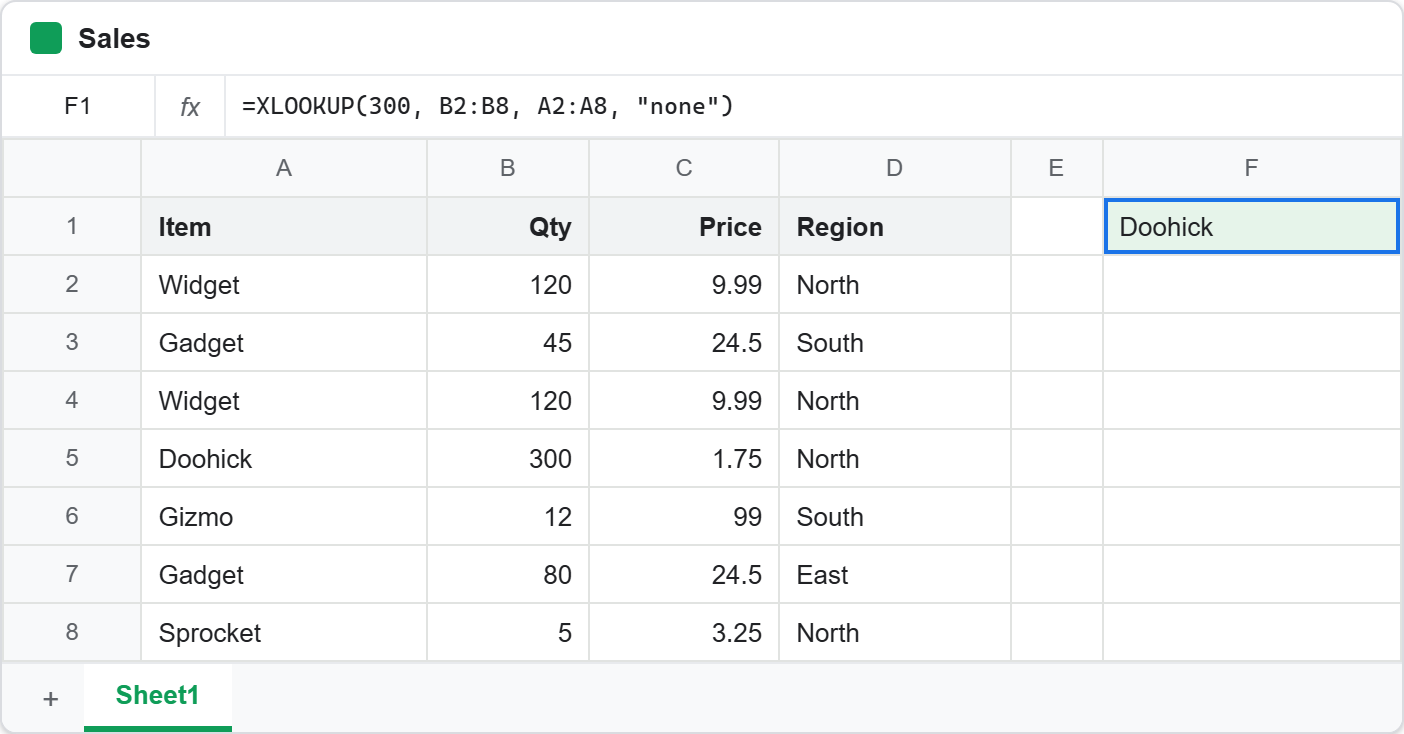
=XLOOKUP(300, B2:B8, A2:A8, "none")
The search range is column B and the return range is column A, to its left. VLOOKUP has no way to express this, since its column number counts rightwards from the search column.
=VLOOKUP(300, B2:D8, -1, FALSE)
That attempt returns #VALUE!. A negative column index is not a valid argument, so the usual workaround is to rebuild the table with the key on the left, or to fall back to INDEX and MATCH.
What the XLOOKUP function does that VLOOKUP cannot.
Two more arguments are worth knowing, and both take their default when omitted.
The sixth argument sets the search direction. Pass -1 and the search runs from the bottom, so a duplicate key returns its last row instead of its first.
=XLOOKUP("Widget", A2:A8, D2:D8, "none", 0, -1)The fifth argument sets how loosely the value has to match. Pass 2 and Google treats the search string as a wildcard pattern.
=XLOOKUP("Gad*", A2:A8, C2:C8, "none", 2)Pass -1 instead and a miss falls back to the next smaller value, which is how you band a number into a range. Note one honest caveat here. Google’s documentation expects the search range to be sorted for that mode, and the range used in this article is not sorted, so treat the result as undefined rather than as a feature until you have sorted the data.
When INDEX and MATCH still win.
The older pair does the same leftward lookup perfectly well.
=INDEX(A2:A8, MATCH(300, B2:B8, 0))
Both return Doohick, so this is not a correctness argument. It is a portability one, and there are three cases where the older pair is still the right choice.
Use INDEX and MATCH when the sheet has to travel to an older Excel, since XLOOKUP arrived in Excel 2021 and anything earlier shows a broken formula. Use it when one MATCH result feeds several INDEX calls, because you can compute the row position once and reuse it rather than searching repeatedly. Finally, use it when your team already reads that idiom fluently, since somebody rewrites a formula nobody trusts anyway.
Complete code for the XLOOKUP function.
Every formula from this article, in order.
// Step 2 - the basic lookup.
=XLOOKUP("Gizmo", A2:A8, C2:C8)

// Step 3 - a miss, then a miss with a fallback.
=XLOOKUP("Nothing", A2:A8, C2:C8)
=XLOOKUP("Nothing", A2:A8, C2:C8, "not found")

// Step 4 - return three columns at once.
=XLOOKUP("Gizmo", A2:A8, B2:D8)

// Step 5 - return a column to the LEFT of the search column.
=XLOOKUP(300, B2:B8, A2:A8, "none")

// VLOOKUP cannot express that at all.
=VLOOKUP(300, B2:D8, -1, FALSE)

// Search from the bottom, so duplicates return the last row.
=XLOOKUP("Widget", A2:A8, D2:D8, "none", 0, -1)

// Treat the search value as a wildcard pattern.
=XLOOKUP("Gad*", A2:A8, C2:C8, "none", 2)

// The older idiom, for comparison.
=INDEX(A2:A8, MATCH(300, B2:B8, 0))
Test the XLOOKUP function.
Nothing to install. Click an empty cell, paste a formula, and press Enter.
Click F1 -> paste the formula -> press Enter
Result of the XLOOKUP function.
The basic lookup returns a single number, and the miss cases differ only in their fourth argument.
=XLOOKUP("Gizmo", A2:A8, C2:C8)                  ->  99
=XLOOKUP("Nothing", A2:A8, C2:C8)                ->  #N/A
=XLOOKUP("Nothing", A2:A8, C2:C8, "not found")   ->  not found
Then the multi-column return spills sideways into three cells from one formula.
12 99 South
The leftward lookup is the one to compare directly against VLOOKUP, because the same question produces an answer in one case and an error in the other.
=XLOOKUP(300, B2:B8, A2:A8, "none")   ->  Doohick
=INDEX(A2:A8, MATCH(300, B2:B8, 0))   ->  Doohick
=VLOOKUP(300, B2:D8, -1, FALSE)       ->  #VALUE!
Finally the two optional arguments. Searching Widget from the bottom returns North, which is also what a forward search returns here because both Widget rows share a region, so change one region to see the difference clearly. The wildcard matches Gadget and returns its price.
=XLOOKUP("Widget", A2:A8, D2:D8, "none", 0, -1)   ->  North
=XLOOKUP("Gad*", A2:A8, C2:C8, "none", 2)         ->  24.5
When to use the XLOOKUP function.
Make it the default for new work. It needs no column counting, it handles the miss in its own argument list, and it reads left to right in the order you would say it out loud.
Keep VLOOKUP where a file has to stay compatible with older software, which is exactly the case the PhpSpreadsheet article covers: a formula written into an .xlsx by a script has to work wherever that file is opened, and you do not control what that will be. Inside a Google Sheet you do control it, so the newer function is free to use.