Two decimal places on screen and a total that is three cents out is the oldest spreadsheet complaint there is. Number formatting only changed the picture, so the ROUND function is what you actually wanted.
Three functions do the work and they share one shape. ROUND goes to the nearest, ROUNDUP always goes away from zero, and ROUNDDOWN always goes towards it. Each takes the same two arguments.
Money is where this bites first, because a price column carries more decimals than it shows. Invoices, tax lines and unit costs all depend on the stored value, and one formula below settles which value that is.
The ROUND function.
Give it a number, then the count of decimal places to keep.
=ROUND(A2,2)
So 3.14159 comes back as 3.14, and the cell now holds exactly that and nothing more. Half rounds away from zero, therefore 2.5 gives 3 rather than the banker’s 2.
The siblings are one word different. =ROUNDUP(A2,2) and =ROUNDDOWN(A2,2) take the same two arguments, yet they ignore which way is nearest.
None of the three is the same thing as a number format. Formatting only repaints the cell, since the stored value never moves. ROUND replaces that value instead, so two columns that look identical can still disagree by a few cents once you total them.
The second argument takes a minus sign.
This is the part almost nobody meets. The decimal count can go negative, and a negative count rounds to the left of the point instead.
=ROUND(A4,-3)
So 1234567 becomes 1235000, because minus three means the nearest thousand. Likewise minus two gives hundreds, and minus six gives millions.
It is genuinely useful for headline figures, since a chart axis or a summary line rarely wants seven significant digits. Also, zero is a valid count, so =ROUND(A2,0) returns a whole number while keeping it a number.
One more sibling belongs here. MROUND rounds to the nearest multiple of whatever you hand it, so =MROUND(A2,0.05) snaps a price to the nearest five cents.
Result of the ROUND function.
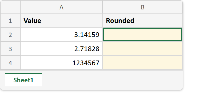
Before. Three values at full precision, with the rounded column still empty.
After. Two ordinary roundings, then the negative-decimals one that moves the digits the other way.
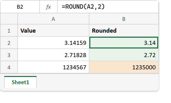
A2  ->  3.14159
A3  ->  2.71828
A4  ->  1234567

=ROUND(A2,2)   ->  3.14
=ROUND(A3,2)   ->  2.72
=ROUND(A4,-3)  ->  1235000
The third line is the one worth remembering. In fact it is the only part of the syntax that catches people twice, once because it is allowed and once because it is useful.
To prove the stored value really moved rather than the display, count what is left with LEN.