TOCOL and TOROW take a rectangular range and return every cell in it as one line: TOCOL gives you a single column, TOROW a single row. Neither moves your data; both produce a reshaped copy that updates when the original does.
That sounds trivial until you need it. A list is what most other functions actually want. UNIQUE, SORT, COUNTIF and every chart in Excel are happier with one column than with a block. So TOCOL and TOROW are how a block becomes one.
This site handles orientation from the other direction too. Write Excel Files Data Horizontally In PHP Using PHPSpreadSheet chooses the layout as the file is written, which is the right moment when a program owns the output. Here the data has already been laid out, possibly by somebody else, and we change our view of it without touching theirs.
One thing decides whether this works or quietly misleads you: the order the cells come out in. That is step 3, and it is worth reading before trusting a result.
Requirements for TOCOL and TOROW:
- Microsoft 365, Excel 2024, or Excel for the web
- A workbook you can edit
- Nothing to install, because TOCOL and TOROW ship with Excel
Excel 2021 is not enough. Dynamic arrays are there, so SORT and UNIQUE work, but the reshaping family arrived in a later wave and Excel 2021 returns #NAME?.
Step 1.
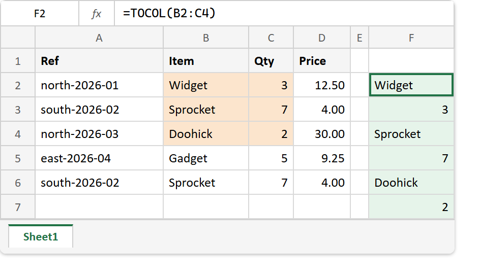
First, lay the table out in A1:D6. We will mostly work with the small block B2:C4, because six cells are easy to follow when the order of the output is the whole point.
Ref             Item      Qty   Price
north-2026-01   Widget    3     12.50
south-2026-02   Sprocket  7     4.00
north-2026-03   Doohick   2     30.00
east-2026-04    Gadget    5     9.25
south-2026-02   Sprocket  7     4.00
Step 2.
Next, flatten the block into one column. One argument, no options.
=TOCOL(B2:C4)
Six cells go in and six come out, stacked vertically. TOROW is the same call with the result turned on its side.
=TOROW(B2:C4)
Consequently a two-column block becomes something a chart or a COUNTIF can consume directly, without a helper column and without rearranging the source.
Step 3.
Now the part that catches people. Both functions read across each row first, not down each column.
=TOCOL(B2:C4)
The result is Widget, 3, Sprocket, 7, Doohick, 2 — names and quantities interleaved, because each row is emptied before the next begins. That is almost never what you want from a table with headings. In fact it is easy to miss entirely, once the two columns hold similar-looking values.
The third argument fixes it. Pass TRUE for scan_by_column and the function empties each column instead.
=TOCOL(B2:C4,,TRUE)
Now the result is Widget, Sprocket, Doohick, 3, 7, 2 — all four names, then all the quantities. Note the empty second argument: the comma has to be there so that TRUE lands in the third position rather than the second.
Step 4.
Then deal with the gaps. The second argument, ignore, takes four values and blanks are the common case.
=TOCOL(E2:F4)
=TOCOL(E2:F4,1)
Using a small block with one empty cell and one #DIV/0! in it, the first returns all six cells and the empty one arrives as 0. That is worth stating plainly. A blank cell in an array does not stay blank — it becomes a zero. Once it does, that zero will happily join an average and change it. Meanwhile 1 drops blanks entirely.
The other two values cover errors.
=TOCOL(E2:F4,2)
=TOCOL(E2:F4,3)
Therefore 2 keeps blanks but discards errors, and 3 discards both. Use 3 when you are feeding the result into a calculation and 0 when you are auditing what is actually in the range.
Step 5.
Finally, compose it. Flattening exists so that the next function has something to chew on.
=UNIQUE(TOCOL(B2:B6))
That returns the distinct item names. Because the flatten happens inside the formula, the source block keeps its shape for the humans reading it while the calculation gets the list it needs.
=ROWS(TOCOL(B2:C4))
Wrapping it in ROWS counts what came out, which is the quickest way to confirm an ignore setting is doing what you think.
What TOCOL and TOROW do that a helper column cannot.
The manual alternative is to build the list once, by hand or with a column of references, and then keep it in step. Three things go wrong with that.
It has a fixed length, so rows added to the source fall off the end silently. It duplicates the data, which means two versions of the truth in one workbook. Finally, it needs maintaining by whoever inherits the file, and that is usually somebody who does not know it exists.
There is also a sibling worth knowing about. WRAPROWS does the reverse — it takes a long list and folds it into a grid of a given width. It is documented alongside these two and belongs to the same family, though it is not covered here.
When leaving the grid alone still wins.
Two cases. First, reshape for a calculation, not for a reader. A flattened column of interleaved names and numbers is unreadable. So keep the block as the thing on screen, and hide the flattened copy. Finally, these functions do not exist in Excel 2021 or older, nor in LibreOffice. While the workbook has to open there, a helper column is the only portable answer.
Complete code for TOCOL and TOROW.
Every formula from this article, in order.
// Step 2 - flatten a block, vertically then horizontally.
=TOCOL(B2:C4)
=TOROW(B2:C4)

// Step 3 - the default reads ACROSS each row; TRUE reads down each column.
=TOCOL(B2:C4,,TRUE)

// Step 4 - the ignore argument, on a block containing a blank and an error.
=TOCOL(E2:F4)      // keep everything; the blank arrives as 0
=TOCOL(E2:F4,1)    // drop blanks
=TOCOL(E2:F4,2)    // drop errors
=TOCOL(E2:F4,3)    // drop both

// Step 5 - flatten so that something else can consume it.
=UNIQUE(TOCOL(B2:B6))
=ROWS(TOCOL(B2:C4))
Test TOCOL and TOROW.
Nothing to install. Click an empty cell, paste a formula, and press Enter.
Click F2 -> paste the formula -> press Enter
Result of TOCOL and TOROW.
The source block and the two flattened versions of it, side by side.
B2:C4          ->  Widget    |  3
                   Sprocket  |  7
                   Doohick   |  2

=TOCOL(B2:C4)  ->  Widget, 3, Sprocket, 7, Doohick, 2   (down one column)
=TOROW(B2:C4)  ->  Widget, 3, Sprocket, 7, Doohick, 2   (along one row)
Then the same six cells with the scan direction switched, which is the comparison the whole article turns on.
=TOCOL(B2:C4)         ->  Widget, 3, Sprocket, 7, Doohick, 2
=TOCOL(B2:C4,,TRUE)   ->  Widget, Sprocket, Doohick, 3, 7, 2
Next the four ignore settings, run against a block holding one blank cell and one #DIV/0!.
=TOCOL(E2:F4)     ->  Widget, 3, 0, 7, Doohick, #DIV/0!
=TOCOL(E2:F4,1)   ->  Widget, 3, 7, Doohick, #DIV/0!
=TOCOL(E2:F4,2)   ->  Widget, 3, 0, 7, Doohick
=TOCOL(E2:F4,3)   ->  Widget, 3, 7, Doohick
Finally the composed forms, which are what you will actually keep in a workbook.
=UNIQUE(TOCOL(B2:B6))   ->  Widget, Sprocket, Doohick, Gadget
=ROWS(TOCOL(B2:C4))     ->  6
When to use TOCOL and TOROW.
Use it whenever a function downstream wants a list and your data is a block. Also, set the scan direction deliberately every time rather than accepting the default. That default suits a matrix of like values. It is wrong for a table of columns that mean different things.
Keep the orientation decision in code when a program writes the file. That is what the PHPSpreadSheet article covers. In that case a script can write the layout the reader needs, and skip the reshaping entirely. Inside a workbook you did not lay out, TOCOL and TOROW give you the shape you need without an argument about whose layout is correct.