Product codes, account numbers and postcodes often carry their meaning in the first few characters. The LEFT function cuts those characters off the front of a cell and hands them back.
In fact, it is the simplest of the text-cutting functions. It takes a cell and a count, and nothing else.
However, what it hands back is always text, even when it looks exactly like a number. That one detail decides whether the next formula works.
The LEFT function.
So give it a cell and the number of characters to keep.
=LEFT(A2,4)
From 1042-UK it returns 1042. Leave out the count and you get one character, so =LEFT(A2) returns just 1. In short, the second argument is optional but almost always wanted.
Also, RIGHT is the mirror image. =RIGHT(A2,2) returns UK from the same cell, and MID takes a piece from anywhere in between.
The result is text, not a number.
Next, add up the numbers you just extracted.
=SUM(B2:B4)
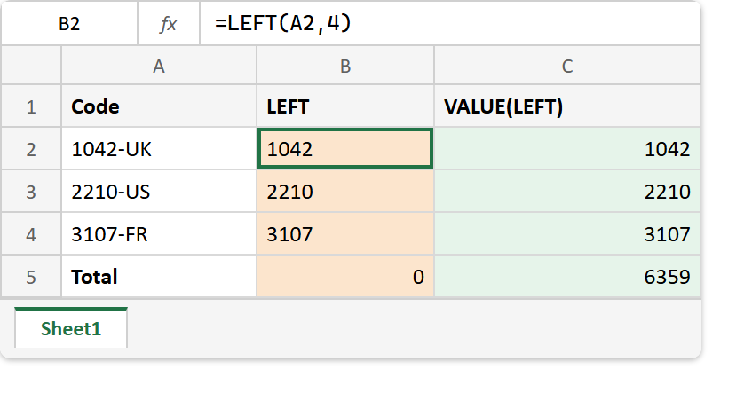
The total is 0. The LEFT function returned the text 1042, and SUM skips text in a range, so it found nothing to add. Notice that the results sit on the left of their cells, which is Excel’s only visual hint.
The fix is to convert as you cut. =VALUE(LEFT(A2,4)) returns the real number 1042, and the same SUM then gives 6359.
Dates hide the same problem more thoroughly. A cell showing 26/09/2026 actually holds the serial number 46291, so =LEFT(A2,4) on it returns 4629, not the year.
Result of the LEFT function.
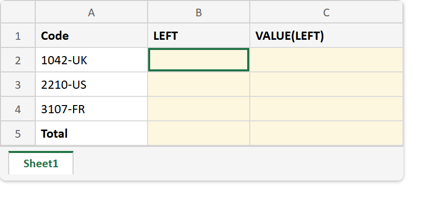
Before. Three product codes, each starting with a four-digit number.
After. The plain LEFT column totals 0, while the column wrapped in VALUE totals 6359.
A2  ->  1042-UK
A3  ->  2210-US
A4  ->  3107-FR

=LEFT(A2,4)          ->  1042    (text)
=SUM(B2:B4)          ->  0       (text is skipped)
=VALUE(LEFT(A2,4))   ->  1042    (number)
=SUM(C2:C4)          ->  6359
=RIGHT(A2,2)         ->  UK
Therefore, wrap the LEFT function in VALUE whenever the piece you cut is meant to be counted. When the piece is not at the start, MID does the same job from any position.