Months end on the 28th, 29th, 30th or 31st, and nobody wants to write that rule out by hand. The EOMONTH function returns the last day of a month for any date you give it.
In fact, it is the quiet engine behind due dates, billing periods and month-end reports. Leap years are handled for you, too.
However, what it returns first is a number rather than a date. That catches almost everyone the first time.
The EOMONTH function.
So give it a date and a number of months to move.
=EOMONTH(A2,0)
A zero means this month, so 26 Sep 2026 gives 30 Sep 2026. Then 1 means next month and -1 last month. In short, the second argument counts months forward or back before finding the end.
Also, February takes care of itself. For 10 Feb 2026 the EOMONTH function returns 28 Feb, and for 10 Feb 2028 it returns 29 Feb.
It returns a serial number, not a date.
Next, type the formula into a fresh cell and look at what appears.
=EOMONTH(A2,0)
You get 46295. That is not an error, because Excel stores every date as a count of days, and 46295 is 30 Sep 2026 in that count. The cell simply has no date format yet.
So format the column as a date and the right answer appears. The value never changed, only the way the cell shows it.
Result of the EOMONTH function.
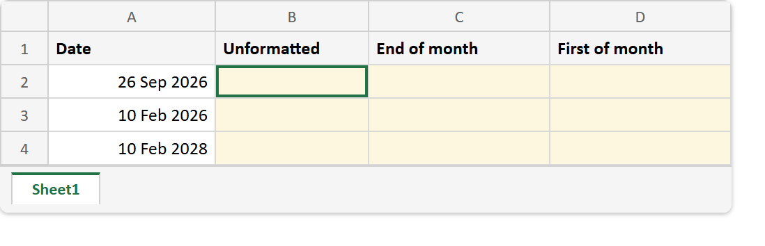
Before. Three dates, including two in February.
After. Raw serial numbers in column B, the same values formatted as dates in column C, and the first of each month in column D.
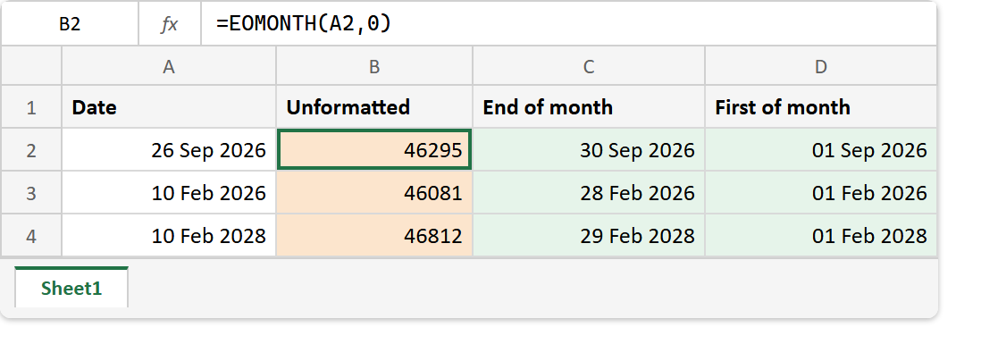
A2 -> 26 Sep 2026
A3 -> 10 Feb 2026
A4 -> 10 Feb 2028

=EOMONTH(A2,0)      ->  46295  ->  30 Sep 2026
=EOMONTH(A3,0)      ->  46081  ->  28 Feb 2026
=EOMONTH(A4,0)      ->  46812  ->  29 Feb 2028   (leap year)
=EOMONTH(A2,-1)+1   ->  01 Sep 2026
=EOMONTH(A2,1)      ->  31 Oct 2026
The most useful line is the fourth. The end of last month plus one day is the first of this month, so =EOMONTH(A2,-1)+1 gives you a clean start date for any period.
Similarly, EDATE moves by whole months but keeps the day, so =EDATE(A2,1) gives 26 Oct 2026. For the serial-number idea from the other side, see TEXT, and for a date that updates itself, TODAY.